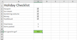
Learning how to create a checklist in Excel is a game-changer for many people. Making a checklist will help you keep track of many everyday things. For instance, a checklist can help you remember what to bring in your travels or the ingredients available when cooking a recipe.

However, not everyone is well-versed in spreadsheets and may find it tough to create a checklist in Excel. This post will discuss how to make a checklist in Excel, plus some pointers on integrating it with other spreadsheet features.

The first step in creating a checklist is coming up with a list of items or activity that needs to be confirmed. Here’s what you should do on the Excel spreadsheet:

1. To open Excel, click on the search button next to the Start menu. Type “Excel” and click on the first result.
2. On a new spreadsheet, type the name of the checklist in one of the cells, preferably in A1, so that it will be easy for you to know what the list is about.
3. Select a column where you will list the items. Then, click a cell where you want to put the first item or activity and type it.
4. Type in the rest of the entries on the succeeding cells of the column. Next, select a column where you are going to put the checkbox. We’ll put it in column B in this example since it’s next to our listed entries. Then, proceed with the instructions below.

How to Use Checkboxes in Excel
Here’s how to make a checkbox in Excel which you can tick to indicate that the entry is completed:

1. Check if you have the Developer tab on the Microsoft Excel toolbar. If not, click File.
2. Scroll down and click Options. Then, click Customize Ribbon.
3. Head to the right side of the panel and tick the Developer box before clicking OK.
4. Click the Developer tab.
5. Click the Insert icon, and under Form Controls, select Checkbox.
6. Select the cell where you want to place the checkbox, preferably next to an entry on your list.
7. You can change the text on the checkbox by deleting the default checkbox text and typing a word or phrase or removing the text entirely so that only the tick box remains.
8. If you want to move the checkbox, drag it to the position you want.
9. To copy the exact checkbox on the succeeding cells, click on it. Then, hover your mouse to the lower right corner of the box and drag it downwards (or to any direction where you want to place the checkboxes).

Important tip: When formatting a checkbox on a cell, hold the Ctrl key and press left-click to modify or resize the shape of the checkbox instead of ticking it.

How to Link Cells in an Excel Checklist

1. If you want to tally the boxes ticked, link the checkbox to another cell.
2. Right-click a checkbox and select Format Control.
3. Go to the Control tab. Head over to the Cell Link option, type the Cell name you want to link. You’ll notice that if you tick the checkbox, the linked cell will display TRUE. Unchecking it will produce FALSE.
4. Repeat steps 1 and 2 to the other cells in the column that must be linked.
5. To get a summary of how many boxes were ticked, click a cell where you want the results displayed. Then, type =COUNTIF(C4:C10,TRUE). Replace C4:C10 with the beginning and ending cells of cell range.
6. If you want to hide the column where the TRUE/FALSE values are displayed, click on the column. Next, press right-click and select Hide at the bottom of the popup menu.

Modify Your Excel Checklist Using Conditional Formatting
Conditional formatting of your spreadsheet can help your data stand out and make it visually appealing.

1. Select the cell you want to modify, then click the Home tab. Go to the right side of the toolbar and click Conditional Formatting.
2. Select New Rule. It will show several rule types which you can use to edit the selected cell. For now, choose Use a formula to determine which cells to format.
3. In the text box below, Edit the Rule Description type =$C4. Next, select Format and then select Fill. Go to Color and change the font color of the cell. Select OK.
4. Notice that when you tick the linked checkbox next to the cell, the text will turn green.
5. Repeat steps 1-4 for the rest of the entries.

Important Tip: Press Ctrl + Shift key and drag the cell to where you want to duplicate the checkbox to produce the same result of copy-pasting. This method will also keep the checkboxes aligned.

How to Make an Interactive Excel Checklist
If you want to track your progress on your recipe to-do checklist, integrate the checklist into a percent of tasks completion. Here’s how you do it:

1. Using the example we currently have, click into any cell where you want to have the task progress to be displayed.
2. Type the following COUNTIF formula =COUNTIF($C$4:$C$10,TRUE). This formula will count the total numbers of entries whose checkboxes were ticked.
3. To track the completion rate of all the entries, type this in the cell where you want it displayed (Example: Cell F4) =COUNTIF($C$4:$C$10,TRUE)/7*100. Note: don’t forget to replace “7” with the number of entries on the list.

For more information on solutions for running your businesses’ technology more efficiently, visit our website or contact Megan Meisner at mmeisner@launchpadonline.com or 813 448-7100 x210.

This was originally posted by OnlinetechTips.